Credit Card Fraud Detection with Machine Learning

Credit card fraud accounts for over a billion €, as stated in a press release by the European Central Bank 🏦. Some of the challenges in detecting fraud is due to the nature of fraud itself, which accounts for less than 0.1% of all transactions. Not only this but also the pattern in detecting financial crime changes over time. Hence, it's no surprise that credit card companies are investing heavily in AI to quickly and easily catch fraudulent transactions.

In this article, I will walk you through how one can set up a simple machine learning detection model on an example dataset of credit card transactions taken from Kaggle. For the Python code, please visit my Github here.

Let's begin!

As always, import all the libraries one is going to need for this project.

# Import libraries

import numpy as np
import pandas as pd
import matplotlib.pyplot as plt
import seaborn as sns
from collections import Counter
from imblearn.over_sampling import SMOTE
from sklearn.model_selection import train_test_split
from sklearn.ensemble import RandomForestClassifier
from sklearn.metrics import recall_score

Here is a preview of what the dataset looks like:

# Load and summarise dataset
df = pd.read_csv('creditcard.csv')
print(df.head(5))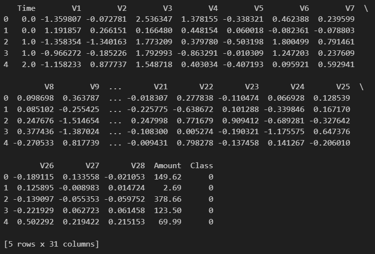

df.info()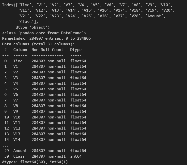

This dataset consists of many predictor variables such as 'Time' and 'Amount'. All other predictor variables (the ones with V prefix) are fields that have been encoded for data privacy purposes. The target variable is the binary field 'Class', which takes either 0 as non-fraudulent or 1 as fraudulent. Since Class is a label of what is fraud and what isn't fraud, then this is a supervised machine learning (ML) problem.

Let's now separate the features from the target into individual matrices as follows:

# Split the dataframe into two matrices, one for all of the features and one for the target variable
X = df.iloc[:, 0:-1]
y = df.iloc[:, -1:]

Then we further divide the two matrices into training and test sets:

# Split the dataset into training and testing sets
X_train, X_test, y_train, y_test = train_test_split(X, y, test_size=0.2)

Running the code below shows the percentage of the dataset that consists of fraudulent transactions.

# Show Class distribution as a pie chart
print("Class as a pie chart:")
fig, ax = plt.subplots(1, 1)
ax.pie(df.Class.value_counts(), autopct='%1.1f%%', labels=['Non Fraud','Fraud'], colors=['yellowgreen','red'])
plt.axis('equal')
plt.ylabel('')

# Calculate % of fraudulent transactions
counter = Counter(df['Class'])
imbalance_ratio = (counter[1]/(counter[0]+counter[1]))*100
print(f"The percentage of fraudulent transactions is {imbalance_ratio}")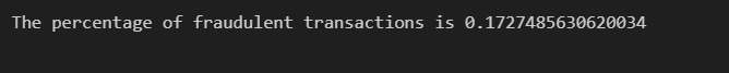

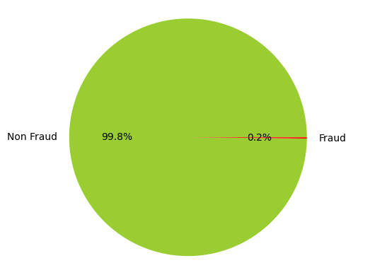
As you can see, the percentage is less than 0.2%, which means it's a very rare occurrence. This kind of pattern is prevalent in many other areas, not just in finance. Hence, it is possible to apply the same approach, say for example, to the detection of cancers.

A visual representation of the skewness in the Class field is shown by running the code cell below:

# Plot Kernel Density Estimate (KDE) to show the imbalance in distribution between fraudulent and non fraudulent instances 
sns.kdeplot(data=y, color='red', fill=True, legend=True)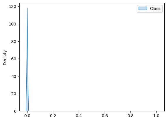

In general, ML algorithms will perform poorly on such a skewed dataset. There are, however, many different techniques used to make such a dataset more "balanced". These techniques are essentially data augmentation techniques, which in a given dataset, just increases the sample of the minority class (oversampling) or decreases the sample of the majority class (undersampling) or both.

One such technique is called Synthetic Minority Oversampling Technique (SMOTE). This technique is different from others, such as random oversampling, because it involves creating a new data point based on it's nearest neighbours in relation to other data points in the minority class in a given feature space. I will delve into more detail on SMOTE in a future article.

Let's employ this technique on our dataset by running the below code cell:

# Over sample the minority class
over_sampling = SMOTE()
X_train_resampled, y_train_resampled = over_sampling.fit_resample(X_train, y_train)

# Plot Kernel Density Estimate (KDE) to show the balance in distribution between fraudulent and non fraudulent instances
sns.kdeplot(data=y_train_resampled, color='red', fill=True, legend=True)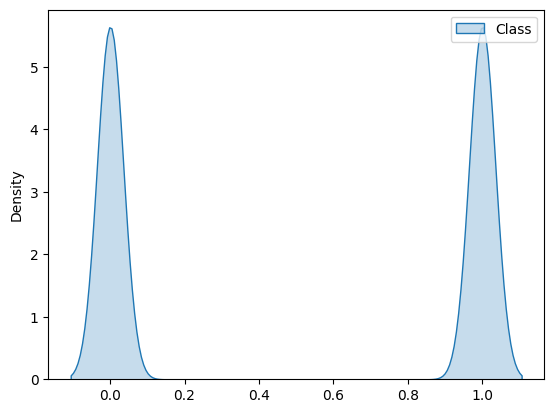

We can see a big difference in terms of the distribution of the majority and minority, with both now being of equal size.

Now, we can get straight into modelling this data, as no data cleaning is needed. Also, I will use all the features within this dataset to train the model as opposed to selecting just a few. This will make the model harder to interpret but the purpose here is to keep it simple for now.

Following the theme of simplicity, we will build a model using the Random Forest algorithm and train it.

# Train model
model_rf = RandomForestClassifier()
model_rf.fit(X_train_resampled, y_train_resampled)

With our model already trained, let's use it to make predictions on the testing set:

# Model prediction on test set
y_pred_rf = model_rf.predict(X_test)

When it comes to evaluating the performance of an ML algorithm for a binary classification such as this one, it is tempting to use accuracy as a metric for performance, especially since it's simple and easy to understand. However, an accuracy score is not appropriate for these kind of problems.

For example, the data set consists of 99.8% of records as non fraudulent and the remainder as fraudulent. If an ML algorithm didn't identify any of the fraudulent transactions, then this model would have an accuracy of 99.8%. Hence, accuracy would be a poor metric for multi-classification problems.

Instead, there is a pair of closely related metrics which are powerful measures of the performance of a ML algorithm for multi-classification problems. These are Precision and Recall. For the purposes of this article, I will use Recall as a measure of model performance, as this is useful for when false negatives are costly, which is the case in credit card fraud.

In a later article, I will delve deeper into the concepts of Precision and Recall but suffice to say for now, Recall is defined below as:

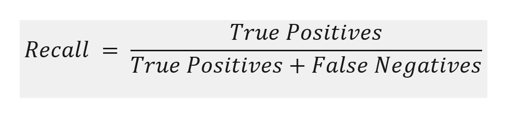
Recall is a measure of the rate at which an ML algorithm correctly predicts true positive instances out of all the actual positive instances. It can take a value between 0 and 1, where the higher the better.

Let's evaluate the Recall score of our Random Forest model:

# Evaluate how often an ML algorithm correctly predicts fraudulent transactions in all cases
r_score_rf = recall_score(y_test, y_pred_rf)
print(r_score_rf)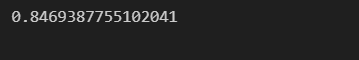

The result is a Recall score of 85%. With minimal effort, we managed to detect 85% of all the fraudulent transactions, which sounds like a good score. Imagine what could be achieved if we spent a bit more time fine tuning the model and carefully selecting a few, strongly correlated features. More on this in another article.

Conclusion

In this article, we covered multiple different aspects of a binary classification problem, specifically where the dataset is imbalanced as is the case in credit card fraud. We covered the SMOTE technique as a way to make the distribution in the Class evenly balanced and also Recall as a metric for evaluating the performance of ML algorithms. These techniques can be applied to many different applications of a similar nature.

If you enjoyed this article and would like see more content like this, then please subscribe using the form below 😄